Field notes / Experiment guide
How much of the exponent spread belongs to the rule?
The census shows a distribution of growth exponents. Is that mostly a difference between rules, or variation between starting patterns?
New to these ants? Start here.
An ant moves on a grid of coloured squares. Each colour tells it to turn left (L) or right (R). It advances that square to the next colour, then steps forward. A rule such as RLR is the list of turns, starting at colour zero. On a blank grid the same rule always makes the same trajectory.
Territory means every cell visited so far. Its boundary consists of visited cells with an unvisited neighbour. A highway is a repeating pattern of motion that carries the ant away. A tether means repeated returns to a small home region.
Growing like the cube root of time means taking eight times as many steps to double a linear size. The rotor walker is a comparison model that follows and rotates arrows stored on cells. A seed makes a random starting pattern reproducible; the ant itself can still move deterministically.
We distinguish c, the chance of discovering a cell per boundary step, from kappa (κ), time at the boundary normalized by perimeter divided by area. Explaining their values is harder than using them to account for growth.
A closer look
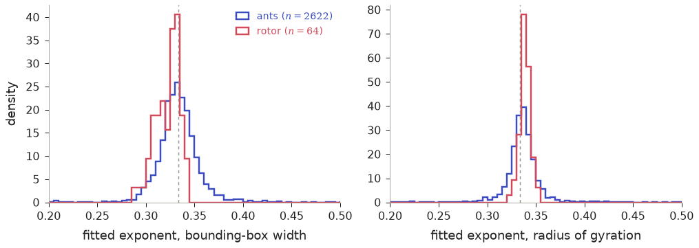
The idea under test
Repeated starts can separate persistent rule differences from seed-to-seed and finite-time variation.
What we learned
Width-exponent variation has a modest rule-level component under both patched and sparse-background starts; area exponents retain more between-rule structure.
What this leaves open
Width and area need not tell the same story when filling fraction and shape change. The windows remain finite.
Read the evidence and reproduction recipe ↗
Inside the experiment
Methods, registered predictions, exact commands and saved analysis. These are the working research documents; expand them for the detail behind the introduction.
Methods and original experiment record
b2-between-rule-variance
Migrated legacy investigation (2026-10-14). Its files used to sit in the flat data/ directory (and calib/, occ/, snaps/, dumps*, knock* where listed) with the label prefix below; experiments/_migration/map.tsv gives the exact old -> new path of every file. This stub was generated from file names and script docstrings. It is not the original write-up: the question, timestamped hypotheses, commands and results are in notes/ (mainly notes/frontier-results.md, notes/frontier-status.md, notes/research-frontier*.md; search for the label), and the producing command is usually in the script docstring or a run_*.sh here.
Old labels / prefixes: b2, b2b, run
Scripts
scripts/b2_anova.py: Within-rule vs between-rule scatter of fitted exponents.scripts/b2_sample.py: B2: 100 random non-bursty blob rules (numpy seed 20261013), disjoint from the 40 rules of experiments/2026-10-13-patched-starts/results/patched.csv, 12 patchedscripts/b2b_anova.py: Within-rule vs between-rule scatter of fitted exponents.scripts/run_b2b.sh
Results
14 entries in results/ (5 are .log/.done markers); csv/json/txt outputs, *_stats.txt hold the summaries quoted in the notes.
Notebook
No committed Jupyter notebook is available for this experiment yet.