Making kappa a consequence

The question that started this experiment was direct: how can we understand κ better, when a theoretical explanation keeps escaping us?

My preliminary answer was that we should try to make κ a consequence. Predict what happens during an ant’s journeys away from the boundary, then ask whether those journeys account for the boundary occupation we actually observe.

That sounds perilously close to something we have already done. It is. The difference has to be made precise, or this experiment will produce another well-measured identity.

What the failures have bought us

κ compares the fraction of steps on the boundary with the boundary’s share of the visited territory. It asks whether the ant uses the edge more or less than uniform occupation would suggest. The probe’s time-window convention complicates that comparison: it divides a window average by an endpoint geometry. The uniform-reference experiment documents the correction. A theory must reproduce that convention.

In the discussion, I initially stressed the prefix result: related opening strings predict related κ values, but the tested models fail on unseen six-letter families. The family hold-out record contains the folds, seed, uncertainty and failures. This does not prove that rule letters lack physical meaning. It tells me that a successful lookup is not yet a portable explanation.

Reading further changed my emphasis. The tail-budget experiment has already tested independent return-time prediction. Its joint criterion failed; its size extrapolation passed its threshold but was beaten by simply carrying the earlier occupation forward. Its parametric tail fit also failed calibration. We cannot start afresh by pretending those tests were never run.

The new proposal therefore has to earn its complexity: can shorter, spatially defined crossing dynamics compose into an accurate long-return law?

The equation that is useful precisely because it explains nothing

Imagine boundary episodes of duration D alternating with interior excursions of duration T. If representative, stable means exist, the long-run boundary fraction is

f_∂ = E[D] / (E[D] + E[T]).

This is a budget identity. Measuring the two means on a trajectory and recovering its occupation would be a check on the accountant. It would not tell us why one rule spends longer away.

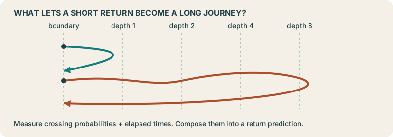
But the equation points to an object we might explain: the survival probability S(t), meaning the chance an interior excursion has not returned by time t. The mean excursion length is the sum of those survival probabilities. A short median tells us little about that sum. Most excursions can be brief while rare continuations consume substantial time.

My working hypothesis is that the field written by the ant controls the chance of those continuations. Two ants might make similar ordinary returns but differ in how often they get past successive depth surfaces.

A scaling relation we can try to break

Let L = A/P, a territory length scale. Suppose, above the short-return regime, the survival law has the form

S(t) ≈ a t^−θ F(t/τ),   τ = b L^z.

The amplitude a says how much probability reaches the tail; τ sets its cutoff. For 0 < θ < 1, integrating this tail gives a contribution to E[T] proportional to a τ^1−θ. Both amplitude and cutoff matter.

If the tail dominates, its shape and amplitudes stabilize, and boundary dwell scales as L^δ, the resulting prediction is

d log κ / d log L ≈ 1 + δ − z(1 − θ).

In my first answer I assumed constant dwell, δ = 0. The protocol makes that assumption measurable rather than silently imposing it. Constant κ then requires z(1 − θ) = 1 + δ. The candidate θ = 1/2, z = 2, δ = 0 satisfies the relation. It has not been measured here.

Try the scaling assumption

Illustrative model only. No ant data. The curves show the tail-dominated approximation κ(L)/κ(L₀) = (L/L₀)^{1+δ−z(1−θ)}. Amplitudes cancel in this ratio.

Candidate: θ = 0.50, z = 2.00, δ = 0.00. Predicted drift is 0: κ stays constant.

For constant dwell and z = 2: θ = 0.25 predicts κ ∝ L⁻⁰·⁵; θ = 0.50 predicts a plateau; θ = 0.75 predicts κ ∝ L⁰·⁵. A plateau alone does not identify the mechanism or predict κ's absolute value.

The attraction is that this proposal can fail in several useful ways. The tail may not have a single cutoff. Its amplitude may drift. Short returns may dominate the mean. Boundary dwell may change with size. Or the exponent relation may hold while the predicted coefficient is wrong. A visually convincing collapse would not settle those questions.

The experiment has to predict the long journey from shorter ones

We will record first crossings between depths 0, 1, 2, 4, 8 and onward, together with their elapsed times. A reduced model starts with depth and arrival direction. We then add heading and colour phase, followed by a local field patch and limited crossing history.

Those measurements define a proposed semi-Markov model: probabilities of the next crossing and the time it costs. Solving its first-return equations gives a return-time prediction. We will compare that prediction with fresh starts, then ask whether the model survives withholding whole rule families.

Those are different tests. Using an unfamiliar start of a familiar rule is not the same as predicting an unfamiliar family. Even the entry distribution and boundary dwell of an unseen family must be predicted without borrowing that family’s measurements.

I am particularly interested in what happens when we enlarge the patch. If predictions stabilize, a local theory becomes plausible. If more distant history keeps changing the answer, that tells us what the small model omitted. It would give us grounds to investigate collective organization of the field.

There is a useful mathematical precedent in random walks with local memory: for the models studied there, the authors characterize a stationary environment as seen from the walker. Their result does not transfer automatically to our ants. It does suggest a productive change of viewpoint: study the field states the walker actually encounters, rather than average all field states equally.

What would change my mind?

I do not want to explain boundary under-occupation by merely saying “slow diffusion.” On a fixed domain, multiplying a uniform-preserving generator by a constant changes the clock without changing stationary occupation. We need a specific asymmetry in returns, residence weights, moving-boundary coupling, or correlations between the walker and its field.

The strongest objection to my preferred story is that the proposed kernel could hide the entire problem in its deepest return time. If almost all of the predicted budget is a measured journey from the deepest milestone back, we have compressed the labels without explaining the journey. The protocol requires reporting that contribution.

Another objection is that depth itself moves. An apparent inward crossing can occur because the boundary moved outward. We will label geometry-induced crossings and compare evolving with frozen contours. A large disagreement blocks the quasi-static interpretation.

Finally, an unfinished excursion can be arbitrarily long. A small number of censored episodes does not guarantee a small error in their mean. Unresolved bounds that permit opposite verdicts make a test uninformative.

What we hope to have at the end

The immediate deliverable is modest: an independently tested return model that beats occupation persistence, identifies where local state is sufficient, and predicts whether κ should flatten or drift. A later intervention could alter the field structure the model identifies and test its predicted response. That causal test needs its own registration.

I would count a clear failure as progress if it tells us where the missing information lives. What I would not count is recovering κ from the same trajectory’s time budget and giving the identity a mechanistic name.

The experiment scaffold and pinned protocol record prospective predictions, seed roles, area bands, controls and stopping gates. No instrument or ant measurements have been run for this experiment. The next step is accounting and synthetic calibration, before a feasibility pilot and a frozen confirmation manifest.