Field notes / Experiment guide
What would uniform occupation actually predict?
We normalize boundary time by perimeter divided by area. Should a walker that is uniformly spread over a growing territory therefore have kappa equal to one?
New to these ants? Start here.
An ant moves on a grid of coloured squares. Each colour tells it to turn left (L) or right (R). It advances that square to the next colour, then steps forward. A rule such as RLR is the list of turns, starting at colour zero. On a blank grid the same rule always makes the same trajectory.
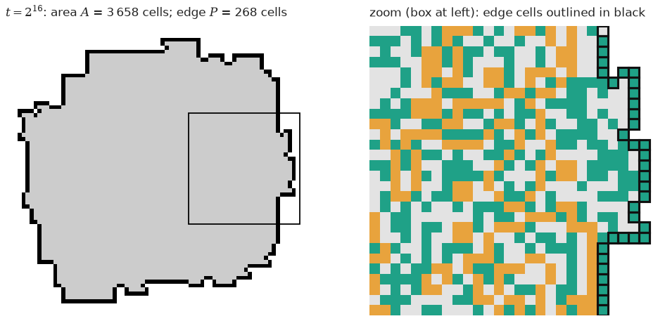
Territory means every cell visited so far. Its boundary consists of visited cells with an unvisited neighbour. A highway is a repeating pattern of motion that carries the ant away. A tether means repeated returns to a small home region.
Growing like the cube root of time means taking eight times as many steps to double a linear size. The rotor walker is a comparison model that follows and rotates arrows stored on cells. A seed makes a random starting pattern reproducible; the ant itself can still move deterministically.
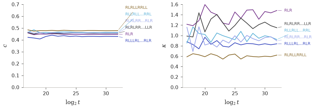
We distinguish c, the chance of discovering a cell per boundary step, from kappa (κ), time at the boundary normalized by perimeter divided by area. Explaining their values is harder than using them to account for growth.
A closer look
The idea under test
Because the probe averages over an expanding time window, the uniform reference must account for growth within that window.
What we learned
The corrected reference differs from one. This changes the baseline against which the ant’s boundary occupation should be compared.
What this leaves open
The calculation is conditional on the assumed growth and geometry. A deviation from the reference does not by itself identify a return mechanism.
Read the evidence and reproduction recipe ↗
Inside the experiment
Methods, registered predictions, exact commands and saved analysis. These are the working research documents; expand them for the detail behind the introduction.
Methods and original experiment record
kappa uniform baseline: what does the probe report for a walker that is uniform by construction?
Registered 2026-10-16 00:25 +13:00, base commit 997c9b2 (dirty workspace from other experiments), before any run.
Question
The paper reads kappa < 1 as "less edge time than uniform" and kappa > 1 as "more". But the probe's kappa = (B/S)/(P_end/A_end) divides window-averaged boundary occupation by the end-of-window edge fraction, while A and P grow through the octave. So a walker with instantaneous occupation ratio exactly 1 need not give probe kappa = 1. What value should be called "uniform"?
Analytic prediction (registered)
If the walker is uniform over the territory at every instant, P(t)/A(t) ∝ A^(β-1) with P ∝ A^β, A ∝ t^a. In the octave (t/2, t], B/S = mean of P/A, so
kappa_unif(a, β) = 2 ∫_{1/2}^{1} x^(-a(1-β)) dx.- smooth blob (β = 1/2), a = 2/3: kappa_unif = 3(1 - 2^(-2/3)) = 1.1102
- β = 1/2, a = 0.95: 1.1587 (diffusive-ish memoryless walker)
- a = 1 (no deceleration, β = 1/2): 1.172
- Only a window starting at t = 0 would give 1.5; not used here.
Mean-field walker (registered)
Each step: resample position uniformly over the currently visited cells, then step to a uniform random 4-neighbour (entering fresh ground if that neighbour is unvisited). Instantaneous occupation of edge cells is then exactly P/A in expectation. The probe's bookkeeping is reproduced inside the example (same Region logic, octave windows (2^k, 2^(k+1)], same definitions of B, P, A), because the probe owns the walker position and cannot teleport.
Predictions:
- Area slope a (fit over k = 12..22) in 0.62–0.72, if P ∝ sqrt(A) holds. If it falls outside, the mean-field territory is rough (β > 1/2) and the analytic kappa must be recomputed with the measured a and β, not 1.11.
- Probe kappa within 0.03 of kappa_unif(a_measured, β_measured), where β is fitted from the same run's (A, P) pairs. Disagreement larger than that means my reading of the probe's kappa is wrong, and is the finding.
- Consequence if confirmed: the ant's reported kappa ≈ 0.9 is a deficit of about 0.9/1.11 ≈ 0.81 relative to uniform, the memoryless walkers' 1.3–1.45 are 1.2–1.3 times uniform, and the rotor's 2.0 is 1.8 times uniform.
Seeds 2026101601..2026101608, board 4096, 2^23 steps (a position list gives O(1) uniform sampling). Mean and between-seed sd reported.
What this does not do
It does not explain the ant's kappa level. It only fixes the reference value. Accounting, not mechanism.
Commands
See NOTEBOOK.md and results/ (filled in as it runs).
Results (2026-10-16 00:41 +13:00)
Command: cargo run --release --example kappa_uniform_baseline -- 2026101601 8 23 results/mf_walker.csv; uv run scripts/analyse.py (output results/analysis.txt). Windows k = 12..22, 8 seeds.
| quantity | prediction | measured (seed sd) |
|---|---|---|
| area slope a | 0.62–0.72 | 0.677 (0.005) |
| perimeter exponent beta | ~0.5 | 0.520 (0.007) |
| probe kappa | 1.107 (formula, measured a, beta) ±0.03 | 1.118 (0.009) |
Predictions 1 and 2 held. The probe's uniform reference is ~1.11, not 1. Restated against it, the ant's ~0.9 is ~0.81× uniform (the rotor and memoryless ratios were not recomputed with their own a, β). Accounting only: the ant's kappa level and the drift remain unexplained.
Notebook
No committed Jupyter notebook is available for this experiment yet.
Read the dated lab log
Lab notebook:
Append-only. Newest entry last. Never edit an old entry; correct it with a new one
(corrects: <timestamp>). Tags: intent, assumption, observation, interpretation,
surprise, decision, dead-end, question, deviation. See experiments/README.md.
YYYY-MM-DD HH:MM (+TZ) · · intent
What I am about to do, why, and which decision it informs.
YYYY-MM-DD HH:MM (+TZ) · · assumption
Statement. How it could be checked / what would show it false. Status: untested.
YYYY-MM-DD HH:MM (+TZ) · · observation
Fact, with the command and file that produced it.
YYYY-MM-DD HH:MM (+TZ) · · interpretation
What I think it means; confidence; the alternative explanations I have not excluded.
2026-10-16 00:25 (+13) · 997c9b2 · intent
Goal: explain kappa. Advisor-guided first step: establish what "uniform" kappa is under the probe's windowing (window-mean B/S over end-of-window P/A). Prediction 1.110 for a=2/3, beta=1/2 registered in README before any run. Informs how to restate the ant 0.9, memoryless 1.3-1.45, rotor 2.0.
2026-10-16 00:26 (+13) · 997c9b2 · observation
src/probe.rs: B counts steps starting on a visited cell with >=1 unvisited 4-neighbour (holes included); P and A are read at window end; windows (2^k,2^(k+1)]. Confirms kappa is window-mean over end-value. Existing "memoryless" walker kappa 1.31 (E1c) was a different, non-teleporting walker, so no uniform baseline existed in notes.
2026-10-16 00:41 (+13) · 997c9b2 · observation
Ran cargo run --release --example kappa_uniform_baseline -- 2026101601 8 23 results/mf_walker.csv (8 seeds, 2^23 steps, board 4096) then uv run scripts/analyse.py -> results/analysis.txt. Mean-field walker: area slope a=0.677 (seed sd 0.005), perimeter exponent beta=0.520 (sd 0.007), probe kappa 1.118 (seed sd 0.009, windows k=12..22, range 1.103-1.139). Formula with measured (a,beta): 1.107; with (2/3,1/2): 1.110. Registered predictions 1 and 2 both held (difference 0.011 < 0.03).
2026-10-16 00:43 (+13) · 997c9b2 · interpretation
The probe's kappa for a walker with instantaneous edge-occupation ratio exactly 1 is ~1.11-1.12, not 1, because B/S is a window mean while P/A is read at window end and A,P grow during the octave. Reference for restating: ant ~0.9 is ~0.81x uniform; memoryless 1.3-1.45 about 1.2-1.3x; rotor 2.0 about 1.8x (rotor/memoryless used their own a, beta only approximately; not recomputed). Caveat: a uniform-on-territory walker is one idealisation; "uniform" could also be taken as uniform over visits-weighted area. This is accounting, not mechanism: the level of the ant's kappa remains unexplained.
2026-10-16 00:44 (+13) · 997c9b2 · decision
Stop at the baseline. The four mechanism plans (tail budget, prefix exposure, gates, field age) are blocked by failed reserve gates / missing checkpoints and are not worth rushing here.
2026-10-16 00:58 (+13) · 997c9b2 · observation
Estimator check (advisor-prompted): experiments/_lib/analyse_probe.py:18-26 forms kappa = (boundary_steps/steps)/(perimeter/area) per octave with steps = t//2 (window length) and P, A at window end; the paper reports the last octave. Same estimator as scripts/analyse.py, single octave, not pooled. So the ~1.11 reference applies to the paper's kappa. Not run through analyse_probe.per_rule itself (schema rename not done).
2026-10-16 00:59 (+13) · 997c9b2 · observation
Added brute-force recount of area and boundary count (two ways) at the end of every mean-field run; assert passes on all 8 seeds. unused_mut warning cleared. Reran: results unchanged (analysis numbers identical). sha256 examples/kappa_uniform_baseline.rs = ffde79de...ac8; results/mf_walker.csv = 94bc152e...260d48 (full hashes: run sha256sum).
2026-10-16 01:00 (+13) · 997c9b2 · deviation
corrects: 2026-10-16 00:43 interpretation. The rotor (1.8x) and memoryless ratios used the 1.11 reference although those walkers have different a (memoryless a~0.95 gives ~1.16, so 1.3-1.45 is ~1.1-1.25x). Only the ant ratio (a~2/3) is justified; treat the rotor/memoryless ratios as unrecomputed. Also not done: notebook.ipynb, tail-budget estimator calibration on this walker, and any mechanism test. Goal (explain kappa level) is NOT met.
2026-10-18 (+13) · 8266186 · observation
Checked the spread of census kappa before treating "0.81x uniform" as a derivation target. scripts/census_spread.py -> results/census_spread.txt (probe_summary.csv, cls == blob, single run per rule). Stationary rules (|g_k|<0.05, n=2185): kappa q05/25/50/75/95 = 0.49/0.73/0.90/1.06/1.47, sd ln kappa 0.35 (0.59 over all 2630). kappa_unif(a,beta) is 1.105 with sd ln 0.004, so the reference is effectively one number. kappa/kappa_unif: median 0.814, geometric mean 0.792, q05..q95 = 0.44..1.33, and 20% of stationary rules are >= 1.
2026-10-18 (+13) · 8266186 · decision
The 0.81 is the median of a wide rule-dependent distribution, not a constant. The target is the distribution (location plus spread), not one number. A derivation of the median alone would not be falsifiable on its own: median and geometric mean differ (0.81 vs 0.79), and single-run noise inflates the observed spread. Does NOT show a universal constant is absent; it shows the data do not call for one.
2026-10-19 (+13) · 8b290d8 · observation
Window labelling note from 2026-10-19-kappa-walker-reference (no change to any number here). This experiment's own CSVs label windows by their start, so "k = 12..22" has window ends 2^13..2^23; the probe CSV's t/k columns label by window end (window (t/2, t]). Same estimator, one octave apart in label. Using t as the start for probe CSVs halves kappa (that experiment caught and fixed this). Also: the census kappa is the last window (k = 26) of analyse_probe.py, not a window mean.