Field notes / Experiment guide
How random is the ant inside its own territory?
A deterministic ant often looks like a random walker in the interior. Do its colours, turns and short-lag motion support that picture?
New to these ants? Start here.
An ant moves on a grid of coloured squares. Each colour tells it to turn left (L) or right (R). It advances that square to the next colour, then steps forward. A rule such as RLR is the list of turns, starting at colour zero. On a blank grid the same rule always makes the same trajectory.
Territory means every cell visited so far. Its boundary consists of visited cells with an unvisited neighbour. A highway is a repeating pattern of motion that carries the ant away. A tether means repeated returns to a small home region.
Growing like the cube root of time means taking eight times as many steps to double a linear size. The rotor walker is a comparison model that follows and rotates arrows stored on cells. A seed makes a random starting pattern reproducible; the ant itself can still move deterministically.
We distinguish c, the chance of discovering a cell per boundary step, from kappa (κ), time at the boundary normalized by perimeter divided by area. Explaining their values is harder than using them to account for growth.
A closer look
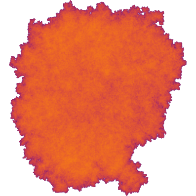
The idea under test
Repeated visits may mix local colour states enough to produce approximately diffusive short-time motion.
What we learned
The mixing diagnostics test local colour, turn and displacement statistics rather than inferring randomness from a picture.
What this leaves open
Short-lag diffusion and colour balance do not establish uniform spatial occupation or explain access to the moving boundary.
Read the evidence and reproduction recipe ↗
Inside the experiment
Methods, registered predictions, exact commands and saved analysis. These are the working research documents; expand them for the detail behind the introduction.
Methods and original experiment record
mixing
Migrated legacy investigation (2026-10-14). Its files used to sit in the flat data/ directory (and calib/, occ/, snaps/, dumps*, knock* where listed) with the label prefix below; experiments/_migration/map.tsv gives the exact old -> new path of every file. This stub was generated from file names and script docstrings. It is not the original write-up: the question, timestamped hypotheses, commands and results are in notes/ (mainly notes/frontier-results.md, notes/frontier-status.md, notes/research-frontier*.md; search for the label), and the producing command is usually in the script docstring or a run_*.sh here.
Old labels / prefixes: mix, mixing
Scripts
scripts/mixing_calib.py: Item 2 calibration: run mixing.py's MSD-slope estimator on a walker whose answer isscripts/mixing_stats.py: Summarise the mixing test (experiments/2026-10-13-mixing/results/mixing.csv) for the page.
Results
6 entries in results/ (0 are .log/.done markers); csv/json/txt outputs, *_stats.txt hold the summaries quoted in the notes.
Notebook
No committed Jupyter notebook is available for this experiment yet.